In a previous post (here) Dr M explained what the NVC is and how to “do” an NVC survey by collecting quadrat data from representative samples in homogenous stands of vegetation.
Here Dr M outlines the procedure for putting an NVC name to your quadrat data.
Now, Dr M assumes you have collected your quadrat data, at least five quadrats in each homogenous stand of vegetation.
Then to identify the closest matching NVC vegetation type(s) the first step is to collate the data into a spreadsheet, with species in the first column and all the quadrats in subsequent columns.
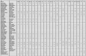
Here is the spreadsheet of data collected by Dr M’s University of Reading MSc Plant Diversity and MSc SISS students:
Click the link to see a pdf of the full dataset Grassland data 2015
Then you need to check the data twice and decide if your plant ID is naughty or nice – we had to correct a misidentified species and delete one column which had been entered twice by mistake, double-checking data is an ABSOLUTE MUST!
These are the raw data, the plan is to reorganise the data by shuffling the rows and columns in a structured way to create a phytosociological table which groups the quadrats into similar vegetation types and groups the species into those which occur together in the vegetation types.
Species frequency – Constancy
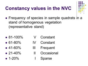
The first step is to calculate species frequency – which in NVC-speak is called “constancy”. A species which occurs in 4 or 5 out of 5 quadrats (or 61-80% of quadrats if you have sampled more than 5) are called a class IV and V constants respectively (Roman numerals are used for constancy classes) and these species are referred to as the “constant” species for that vegetation. Constant species are a big deal in the NVC and really define the vegetation as they are the species you encounter again and again in a particular vegetation type.
A species which occurs in 3 out of 5 quadrats (or 41-60% of quadrats if you have sampled more than 5) are called a class III constants and these species are referred to as “frequent” species in that vegetation.
Similarly species occurring in 2 out of 5 quadrats (or 21-40% of quadrats if you have sampled more than 5) are called a class II constants and these species are referred to as “occasional” species.
Finally, species occurring in 1 out of 5 quadrats (or 1-20% of quadrats if you have sampled more than 5) are called a class I constants and these species are referred to as “sparse” species.
Species abundance – Domin range
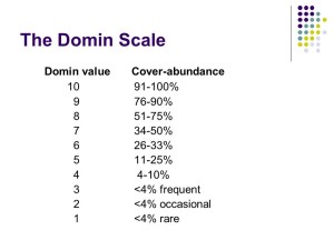
The next step is to calculate the range of abundance for each species in the different quadrats (we call this “the Domin range”).
Once you have calculated constancy values for each species you reorder the data in the spreadsheet by constancy so the class V constants are at the top of the sheet, and the class I species at the bottom.
- Site 1 raw data
- Site 1 reordered by constancy and Domin range
After this, you reorganise the species within constancy classes using the Domin range so species with highest abundance are at the top of the list for that constancy class, and the least abundant species are at the bottom.
Check the images above to make sure you follow this procedure, it is vital to do this to create a proper phytosociological table for the vegetation you have sampled.
Next you need to interrogate the raw data matrix, shine a bright torch in its eyes until it tells you what you want to know!
Ok it doesn’t have to be that dramatic or that cruel, there is a gentler way!
There are two gentler ways in fact:
1. Using hard copy keys.
2. Automated procedures using computer software.
In both cases we need to follow up with careful reading of the relevant chapters of the NVC volumes (British Plant Communities).
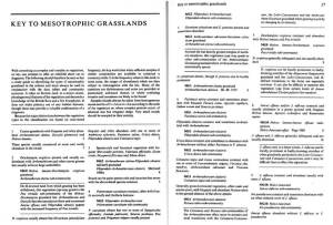
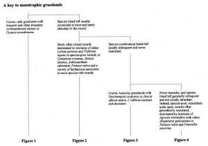
1. Hard copy keys: for grassland vegetation we have the dichotomous keys in the NVC grassland volume (British Plant Communities Volume 3, Rodwell 1992) and also the diagrammatic keys in the summary descriptions of the NVC grassland communities (Cooper 1997).
You will need to check the original publication to see the full versions but here are some extracts:
The first page of the NVC key to mesotrophic grasslands (Rodwell 1992):
The first part of the diagrammatic key (Cooper 1997):
2. Automated procedures using computer software: there are three options: MATCH, TABLEFIT or MAVIS.
Dr M uses MATCH and MAVIS, here we will just consider MAVIS.
MAVIS – Modular Analysis of Vegetation Information System
The MAVIS software can be obtained free from the Centre for Ecology and Hydrology (CEH) and although there are some glitches and irritations (nobody’s perfect!) it is arguably the simplest to use of the available software.
You can download the software from CEH here.
Follow the instructions and remember:
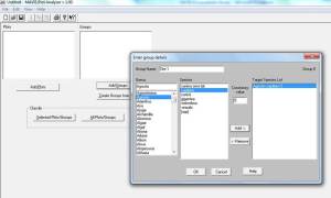
Plots are quadrats (use select plots to input individual quadrats species and % cover (weirdly it is not possible to input DOMIN values even though DOMIN is standard for NVC survey!).
Groups are groups of quadrats e.g. from different sites (use select groups to input species and constancy values).
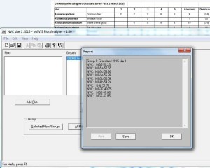
Once you have entered all the data select “classify groups” to get the top ten NVC communities and sub-communities closest to your data.
MAVIS uses the Czechanowski similarity algorithm, to compare your data with all of the NVC community profiles in the NVC database.
MAVIS gives the ten highest coefficients, here are the results for site 1:
A common question is “Dr M, please tell me, which do I choose?” This is an important question!
Sometimes the coefficients can be very similar, so how do you decide between coefficients of say 59.23 and 57.55 as in the example here?
The key point here is not to fixate on the coefficients, actually they cannot easily be interpreted except in broad terms.
Instead, it is better to read the relevant chapter(s) of British Plant Communities for the vegetation you are analysing (grassland in this case) and read the text describing the vegetation of the relevant communities and subcommunities.
Then, it’s up to you to decide which of the top ten is the best fit, and remember, there may NOT be an exact or perhaps even a close match.
You may have atypical vegetation, or something not yet fully described by the NVC (ref to report here) or maybe you did not sample a homogenous stand but perhaps your quadrats straddled two vegetation types or a mosaic of types.
So, in the end you must choose the “answer” which you (as the ecologist) can best justify using the data you have.
If you really can’t find a final answer that you are satisfied with at sub-community level (e.g. MG5a) then just refer to the closest community (MG5).
The next task is to repeat the above for the remaining homogenous stands (sites 2 and 3 in this example).
One thing to remember is to make sure that your the separate set of quadrats your are analysing come from homogenous stands of vegetation.
If you have sampled vegetation across different homogenous stands and analysed them as “one” stand your results will be confused (and so will you be too!).
The best way to check this is to eyeball the spreadsheet and see if there are any quadrats which just look out of place.
If the species lists are similar but with differing abundances then this is probably variation within a vegetation type (maybe a different sub-community).
However if the species lists are quite different then maybe there are different vegetation types mixed together and you need to analyse the anomalous quadrat(s) separately, maybe they belong to one of the other stands you gave sampled or perhaps are something entirely different.


